
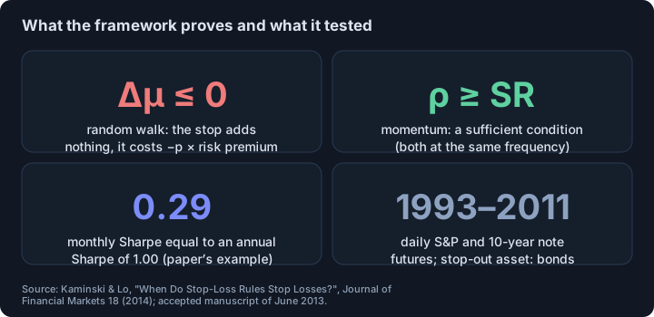
- Short answer: it depends on how returns behave. Kaminski and Lo prove that if returns follow a random walk, a stop-loss always lowers expected return by (stop probability × risk premium); with momentum it can raise it, and a sufficient condition is that autocorrelation is at least the Sharpe ratio at the same frequency.
- Tested on daily S&P 500 and 10-year note futures (1993–2011), stop-losses over short windows had a negative “stopping premium” across wide ranges of parameters; at frequencies above one month some rules added return and cut volatility. The tests ignore transaction costs.
- The rule studied is a portfolio overlay that moves everything into a safe asset, not a protective order on one leveraged trade. In our check, Bitcoin meets the momentum condition only at the weekly frequency and by less than the noise: inconclusive.
- The authors say their findings shed little light on market efficiency versus behavioral finance, and that the success may come from nonlinearities that the rule happens to exploit.
Short answer. Stop-losses are almost universal in practice and almost absent from the early academic literature, and Kathryn Kaminski and Andrew Lo explain why: whether a stop-loss helps depends entirely on how returns behave. If prices follow a random walk, the stop-loss always costs money. If returns have momentum, it can earn money.1
Which kind of stop-loss does the study analyse?
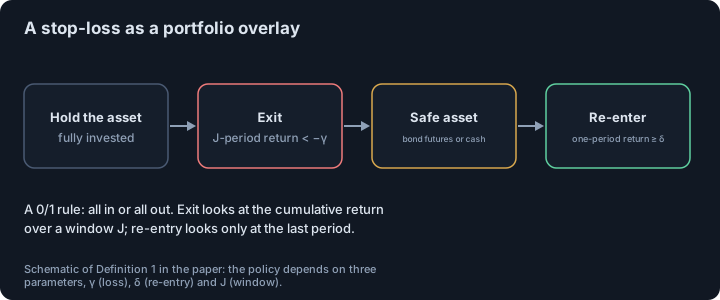
The authors analyse a stop-loss as an overlay on a portfolio strategy: a 0/1 rule that moves 100% from the strategy to a safe asset when the cumulative return over a window of J periods falls below a threshold −γ, and moves back when a one-period return reaches a level δ. The three parameters are the loss threshold, the re-entry threshold and the window.1 The exit and re-entry rules are deliberately different, motivated by loss aversion (becoming less risk-averse when losses mount) and by the “snake-bite” effect (reluctance to re-enter after losses).1
The key quantity is the stopping premium: the expected return of the portfolio with the rule minus the expected return without it. Because the two differ only when the rule is active, it equals the probability of being stopped out times the difference between the safe asset’s return and the portfolio’s expected return during the stop-out.1
What happens if prices follow a random walk?
Proposition 1 gives a strong answer: if returns are independent and identically distributed with an expected return above the risk-free rate, the stopping premium is −(stop probability × risk premium), never positive. Whether the stop is active carries no information about the next return, so the only effect is to swap the portfolio for the safe asset at random times.1 In the authors’ words: “In such cases, stop-loss rules never stop losses.”1
The same proposition shows the effect on risk: the variance change is −p·σ² + p(1−p)·π², so with enough stop-outs and a small enough risk premium the rule can still reduce volatility.1 The authors note that the long dominance of the random-walk view in the 1960s and 1970s may explain why academics gave stop-loss rules little attention, and that their rule resembles the “filter rules” of Alexander (1961) and Fama and Blume (1966), which showed no excess profit.1
What changes when returns have momentum?
For an AR(1) return process with autocorrelation ρ, Proposition 2 gives a first-order result: the stopping premium per unit of stop probability is −π + ρσ plus a remainder that is non-negative for ρ > 0 and reasonable parameters. If ρ is negative (mean reversion) the rule hurts expected returns, because it misses the reversal. If ρ is positive (momentum) it can add value, and a sufficient condition is:1
ρ ≥ π / σ = the Sharpe ratio of the portfolio strategy
Both must be measured at the same frequency. The paper gives an example: a strategy with an annual Sharpe ratio of 1.00 has a monthly Sharpe ratio of 0.29, still a high hurdle for monthly autocorrelation.1
The authors also analyse a two-state regime-switching model, where a stop-loss helps if it detects the low-return state. Fitted to S&P 500 futures it gives a frequent positive low-volatility state (mean 22.3%, volatility 10.3% a year) and a less frequent negative high-volatility state (mean −39.0%, volatility 33.0%).1
What did the test on futures show?
They applied the rule to daily futures from 5 January 1993 to 7 November 2011: the S&P 500 contract as the risky asset (annualized mean 7.3%, volatility 19.5%, Sharpe ratio 0.37) and the 10-year Treasury-note contract as the safe asset (mean 1.2%, volatility 6.3%, Sharpe 0.19); the correlation between them is −17%.1 They tried windows from daily to quarterly (for example 3, 5 and 10 times the sampling interval), loss thresholds between −1.5 and −0.5 standard deviations and re-entry thresholds between −0.5 and 1 standard deviation, deliberately across a wide grid to avoid selecting one setting.1
The results: stop-loss rules at shorter, higher frequencies had negative stopping premiums over large ranges of parameters; at frequencies above one month they performed better and could achieve positive premiums, with higher Sharpe ratios as volatility fell. The exit decision and threshold mattered more than the re-entry threshold. In one calibration, monthly stops on daily data raised return by 1.5% and cut volatility by 5%, lifting the Sharpe ratio by as much as 20%.1 The rolling autocorrelation of the S&P contract swung between momentum and mean-reversion periods, which is the theory’s own warning that the premium is not stable.1
Does Bitcoin meet the momentum condition?
We checked the paper’s sufficient condition on Binance BTCUSDT closes from September 2019 to October 2026, with simple returns and the risk-free rate set to zero. At daily frequency the first-order autocorrelation is −0.066 against a Sharpe ratio of 0.042: not met. At weekly frequency, 0.131 against 0.112: met by a small margin (standard error about 0.05). At monthly frequency, 0.177 against 0.223 (standard error about 0.11): not met, and shifting the start of the 30-day blocks moves it between 0.09 and 0.21.2
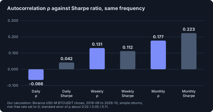
The condition is sufficient, not necessary, and it relies on the paper’s AR(1) approximation. Our result is the honest middle: no clear momentum at the horizons that matter, and not enough data to say. For the base rate of the typical trader, see do day traders make money.
What does the study not say?
- Transaction costs. They are left out (κ = 0), although the authors give the formula and note that more frequent stops mean more trading.1
- Which stop. The rule is a portfolio switch into bonds, not a protective order on one leveraged trade. For what happens around stop orders in the order book, see why price reverses right after your stop is hit.
- Optimization. The rule is a heuristic, not derived from an optimization, and the authors say so.1
- Interpretation. They write that their findings shed little light on market efficiency versus behavioral finance, and that the success may be due to nonlinearities the rule happens to benefit from.1 They also suggest that a systematic rule may profit from the disposition effect; for that bias see why traders cut winners early and hold losers.
- Markets. Daily US index and bond futures, 1993–2011: no crypto, no leverage constraints.
What should a trader take from this?
- A stop-loss is a bet on the return process: it helps in a trending regime and costs in a mean-reverting or random one. State which regime your stop assumes.
- Test stops on a period after the one you chose them on, and include costs; see how many trades you need.
- Expect shorter stops to be worse than longer ones in this evidence, which was positive only above monthly frequencies.
- Do not read the paper as a case for any specific stop distance.
This is educational material, not investment advice.
Related. Why price reverses right after your stop is hit, why you cut winners early and hold losers.
Footnotes
-
Kathryn M. Kaminski and Andrew W. Lo, “When Do Stop-Loss Rules Stop Losses?”, Journal of Financial Markets 18 (2014), 234–254. We read the accepted manuscript dated 28 June 2013 in full (introduction, sections 3–6, Tables 1–2, appendix). Earlier working papers of 2007–2008 used different data (monthly data from 1950); the numbers here are those of the 2013 manuscript, and the journal text may differ slightly. The mean, volatility and Sharpe ratio of Table 1 are annualized with 250 days a year. ↩ ↩2 ↩3 ↩4 ↩5 ↩6 ↩7 ↩8 ↩9 ↩10 ↩11 ↩12 ↩13 ↩14 ↩15 ↩16 ↩17 ↩18
-
Our calculation: Binance USD-M BTCUSDT closes, 2,583 days from 9 September 2019 to 4 October 2026; daily returns, non-overlapping 7-day returns (369) and non-overlapping 30-day returns (86); first-order autocorrelation and mean/standard deviation (Sharpe with zero risk-free rate) at the same frequency; standard error of autocorrelation approximated by 1/√n. Offsets of the monthly blocks by 10 and 20 days gave autocorrelations of 0.09 and 0.21. ↩
Frequently asked questions
Do stop-loss orders improve returns?
It depends on the return process. Kaminski and Lo show that if returns follow a random walk a stop-loss always lowers expected return, but if returns have momentum (positive serial correlation) it can raise it. Their test on futures found positive effects only at longer frequencies and with some parameters.
What is the stopping premium?
It is the expected-return difference between a portfolio with a stop-loss rule and the same portfolio without it. Under a random walk it equals minus the probability of being stopped out times the portfolio’s risk premium, so it is never positive.
When does a stop-loss add value?
In the authors’ AR(1) analysis, a sufficient condition for a reasonable stop-loss rule to add value is that return autocorrelation is at least the Sharpe ratio, both measured at the same frequency. They also show that mean reversion makes stop-losses hurt expected returns.
Does this prove stop-losses work for traders?
No. The paper studies a 0/1 portfolio overlay that moves into bonds, tested on daily index and bond futures from 1993 to 2011 without transaction costs. It does not test protective orders on a single leveraged position or on crypto.
Sources
- When Do Stop-Loss Rules Stop Losses?. Kathryn M. Kaminski and Andrew W. Lo, Journal of Financial Markets 18, 234–254 (2014); accepted manuscript of 28 June 2013 read in full (author copy), 2014
This article is research, not investment advice. Results on history do not guarantee future results.