
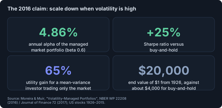
- Short answer: it depends on how you test it. Moreira and Muir (2016) reported that scaling the US market down after a high-variance month gave an annual alpha of 4.86% and lifted the Sharpe ratio by 25% (1926–2015, in-sample).
- Cederburg et al. (2020) tested 103 equity strategies in real time: the managed version had the higher Sharpe ratio in 53 cases and the original in 50, only 8 differences were significant, and a real-time mix did worse than the original in 72 of 103 cases.
- The two papers agree on a premise: volatility is forecastable and does not predict returns much. They disagree on whether you could have traded the gain without hindsight.
- In our BTCUSDT daily data, the day after a move beyond 2 standard deviations had a mean absolute move of 0.96 standard deviations, against 0.64 after other days: the premise holds, but it says nothing about returns.
Short answer. Two respected papers examine the same simple rule and reach different conclusions about whether it pays. The rule: hold less of an asset when its recent volatility is high and more when it is low. The 2016 paper reported large gains; the 2020 paper, built around what an investor could do in real time, found no systematic improvement.12 The practical lesson is about testing, not about the rule itself.
What is volatility targeting?
Moreira and Muir scale each month’s excess return by the inverse of the previous month’s realized variance, written as c ÷ σ²(t−1), where the constant c sets the average exposure; they choose c so that the managed portfolio has the same overall standard deviation as the original.1 Realized variance is the sum of squared daily returns over the previous month; it needs no estimation, so an investor could calculate it in real time.1
The reasoning is the mean-variance rule: the best weight is proportional to expected return divided by variance. Variance is predictable over short horizons, expected return is hard to predict, so the weight should follow the inverse of variance.1
What did Moreira and Muir find?
For the US market portfolio the scaled version had an annualized alpha of 4.86% against the original, with a beta of 0.6, an appraisal ratio of about 0.33 and an overall 25% increase in the Sharpe ratio.1 The authors compute a 65% lifetime utility gain for a mean-variance investor trading only the market, against 35% in earlier work on timing expected returns.1 Their chart shows $1 invested in 1926 growing to about $20,000 for the managed market portfolio against about $4,000 for buy-and-hold, on a nominal log scale.1
They also checked costs and leverage. With a trading cost of 1 basis point, 10 basis points (about 1% of daily volume) and 14 basis points in very high volatility, the alpha fell but stayed large; versions that cap exposure at 1 or 1.5 trade less. An investor under a hard no-leverage constraint, they report, still gets a utility benefit of about 50%.1 Two honest limits appear in the paper itself: alphas were weaker in 1956–1985 because volatility varied less, and if volatility were constant the strategy would be identical to buy-and-hold.1
What did the replication with 103 strategies find?
Cederburg, O’Doherty, Wang and Yan built the same managed portfolios for 103 equity strategies and compared them directly with the originals. Volatility scaling gave a higher Sharpe ratio for 5 of the 9 factors Moreira and Muir studied; across all 103 strategies the managed version won in 53 cases and the original in 50, and only 8 differences were statistically significant in favour of management, concentrated in momentum-related strategies.2
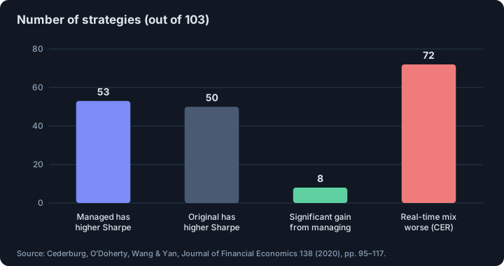
They confirm Moreira and Muir’s regression result: 77 of the 103 managed portfolios have positive alphas (23 significantly positive, 3 significantly negative).2 The catch is what that alpha implies. The regression is equivalent to holding a mix of the scaled and unscaled portfolios with weights chosen using the whole sample, which no investor knows in advance. When the authors form the mix using only past data, it earns a lower certainty-equivalent return than the unscaled portfolio in 72 of 103 cases; they trace this to structural instability in the underlying regressions.2
Why do the two papers disagree?
They measure different things. Moreira and Muir show an in-sample relationship: months of high volatility were followed by returns that did not compensate for the risk. Cederburg et al. ask whether a rule built on that relationship, using only information available at each date, would have beaten simply holding the portfolio. The first can be true while the second fails, because the relationship shifts over time. This is the same distinction as in why backtests lie and in data snooping.
Does the premise hold for crypto?
The premise has two parts: volatility is forecastable, and it does not predict returns much. We can check the first on our data. In Binance USD-M BTCUSDT daily closes (September 2019 to October 2026) there were 140 days with a move larger than 2 standard deviations. The next day’s mean absolute move was 0.96 standard deviations after those days and 0.64 after all other days.3 Volatility clusters. That says nothing about returns: neither paper tests crypto, and we do not claim the rule improves crypto returns.
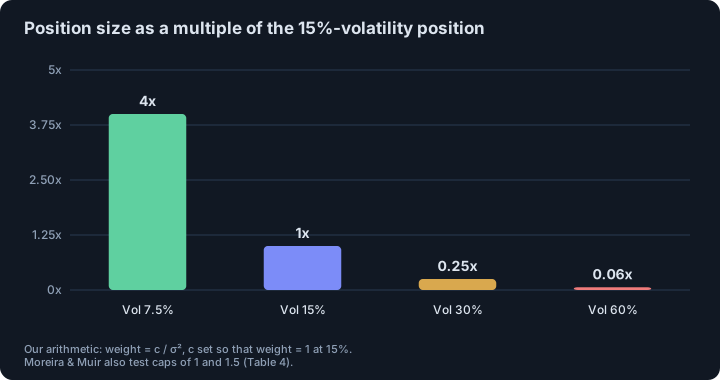
One more caution from the paper’s own mechanics: variance scaling can demand very large swings in exposure. With the position set to 1 at 15% volatility, exposure would be 4 at 7.5% volatility and 0.06 at 60%, our arithmetic. That is why the authors also test inverse-volatility versions and caps at 1 and 1.5.1
What should a trader take from this?
- Reducing size after volatile periods is a risk-control choice, not a proven source of excess return.
- If you test a sizing rule, build it only from past data and compare it directly with the plain version, as the second paper does.
- Expect the benefit, if any, to concentrate where volatility varies a lot, as in momentum-related strategies.
- Cap the leverage of any inverse-variance rule; costs and cap choices matter more than the headline alpha.
- Related sizing logic: Kelly criterion and position size.
This is educational material, not investment advice.
Related. Why backtests lie, Kelly criterion and position size.
Footnotes
-
Alan Moreira and Tyler Muir, “Volatility Managed Portfolios”, NBER Working Paper 22208 (April 2016, revised June 2016), full text read: abstract, sections 1–3 (formula (1)–(2), Tables 1 and 4, Figures 3–4), conclusion. US data 1926–2015; published as Journal of Finance 72(4), 1611–1644 (2017), whose text we did not read. All figures are in-sample and nominal. ↩ ↩2 ↩3 ↩4 ↩5 ↩6 ↩7 ↩8 ↩9 ↩10
-
Scott Cederburg, Michael S. O’Doherty, Feifei Wang and Xuemin (Sterling) Yan, “On the performance of volatility-managed portfolios”, Journal of Financial Economics 138 (2020), 95–117 (full text read: abstract and introduction; counts quoted from the introduction). ↩ ↩2 ↩3 ↩4
-
Our calculation: 2,583 daily log returns of Binance USD-M BTCUSDT closes, 9 September 2019 to 4 October 2026; “standard deviation” is the full-sample standard deviation (3.2% a day); 140 days had an absolute standardized move above 2. ↩
Frequently asked questions
What is volatility targeting?
It means sizing a position inversely to recent volatility: smaller when the market has been wild, larger when it has been calm. Moreira and Muir scale each month’s return by one divided by the previous month’s realized variance.
Does volatility targeting improve returns?
Evidence is mixed. An influential 2016 study found large in-sample alphas, but a 2020 test on 103 equity strategies found no systematic Sharpe-ratio gain and worse out-of-sample results for implementable versions, except in momentum-related strategies.
Why do the two studies disagree?
The alpha in the first study comes from a regression that implicitly uses the best combination of scaled and unscaled portfolios chosen with hindsight. The second study built versions that use only past data and found the weights unstable.
Does it work for Bitcoin?
Neither paper tests crypto. In our BTCUSDT data volatility clusters strongly, which is the premise of the method, but that is not evidence that scaling positions improves returns.
Sources
- Volatility Managed Portfolios. Alan Moreira and Tyler Muir, NBER Working Paper 22208 (April 2016, revised June 2016; full text read); Journal of Finance 72(4), 1611–1644 (2017), 2016
- On the performance of volatility-managed portfolios. Scott Cederburg, Michael S. O’Doherty, Feifei Wang and Xuemin Yan, Journal of Financial Economics 138, 95–117 (full text read), 2020
This article is research, not investment advice. Results on history do not guarantee future results.