
- Short answer: if you tried many variants and kept the best one, its p-value must be computed against the best of all of them, not against itself. Otherwise “significant” mostly measures how hard you searched.
- In Halbert White’s own example, 3,654 linear models for S&P 500 daily returns produced a best model that called the market direction right 54.7% of the time against 50.8% for a constant benchmark. Treated as the only model, its p-value was 0.0036. Accounting for the search, it was 0.2040.
- The correction is a bootstrap that asks how often the best of all candidates would beat the benchmark by this much if none of them had any real skill. White’s paper calls the difference between the two p-values a direct estimate of the data-mining bias.
- It only works on what you record. Every variant you tried, including the ones you discarded, has to be in the comparison.
Short answer. If you tried many versions of a strategy and report the best one, the honest question is not “is this result unlikely by chance?” but “is it unlikely among the best of all the versions I tried?”. Halbert White built a test for exactly that. In his example a model whose p-value looked like 0.0036 on its own had a p-value of 0.20 once the 3,654 models searched were counted, which is nowhere near convincing.
What is data snooping, and why is it hard to avoid?
White starts from a definition:
Data snooping occurs when a given set of data is used more than once for purposes of inference or model selection.
White, “A Reality Check for Data Snooping”, Econometrica (2000)
His point is that in time series there is usually only one history, so reuse is nearly unavoidable.1 Run enough specifications over one price history and some will look good with no real forecasting relation behind them. He compares it to a newsletter scam: send a free tip sheet to many people, half told the market will rise and half that it will fall, keep writing only to those who got the right call, and after a few rounds some recipients have seen a perfect record by construction.
Trading parameter searches work the same way. Moving-average lengths, stop distances, session filters and entry thresholds multiply into hundreds of variants, and the winner of that contest is selected for having been lucky on this sample. We covered the first-order version of this in why backtests mislead.
What did White’s example actually show?
He applied his test to a deliberately ordinary problem: forecasting S&P 500 daily returns one day ahead. He built 29 technical indicators of the kind used by commodity traders (momentum, local trends, relative strength, moving-average oscillators) and fitted every linear model that had a constant plus exactly three of the indicators. That is 3,654 models. The benchmark was a constant alone, which embodies the idea that returns are not forecastable. The evaluation window ran from 3 June 1991 to 31 May 1994, 758 trading days.2
The best model by directional accuracy called the sign of the next day right 54.75% of the time, against 50.79% for the benchmark. That is a gap of about four percentage points, and the two p-values tell very different stories:
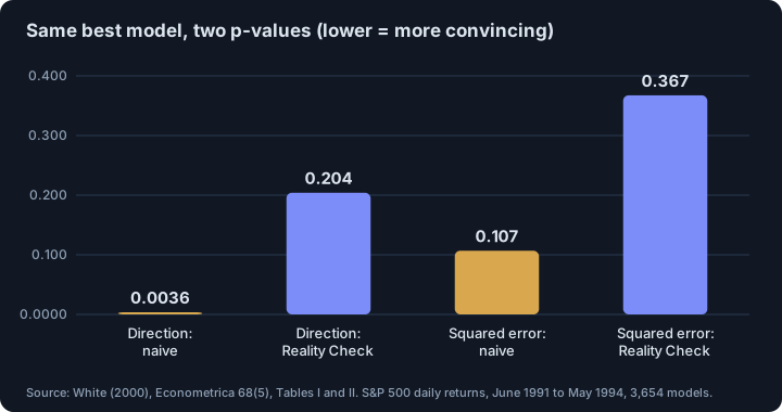
| Criterion | Best model | Benchmark | Naive p-value | Reality Check p-value |
|---|---|---|---|---|
| Directional accuracy | 54.75% correct | 50.79% | 0.0036 | 0.2040 |
| Prediction mean squared error | RMSE 0.006373 | RMSE 0.006410 | 0.1068 | 0.3674 |
White’s own comment on the first row is blunt: “This example dramatically illustrates the dangers of data mining.”2 A p-value of 0.0036 would pass almost any bar a trader would set. Corrected for the search, it is an unremarkable 0.20. The paper also notes that the difference between the two numbers “gives a direct estimate of the data-mining bias”.
How does the Reality Check work?
The null hypothesis is that the best model found in the search has no predictive superiority over the benchmark. The test does not ask how good the best model looks. It asks how good the best of 3,654 would look if none had any skill, and compares your actual best against that.
In practice, for a trader, a simplified version of the idea looks like this (our description of the principle, not White’s full procedure):
- Keep the return series of every variant you tried over the same dates, not only the winner.
- Resample the time axis (in blocks, to keep autocorrelation) and apply the same resampled dates to all variants.
- In each resample, record the best average result across all variants, after centring each variant so that the “no skill” hypothesis holds.
- The p-value is the share of resamples whose best result is at least as good as the one you observed.
White used a stationary bootstrap with 500 resamples for this example.2 Because the whole set is resampled together, the method respects the fact that variants of the same idea are highly correlated, which matters for the next point.
Does searching more always destroy the evidence?
No, and White says so. Candidate forecasts that are highly correlated add little new “chances”; in his figures the p-value stays flat for stretches while correlated models are added, and “consideration of even a large number of models need not lead to dramatic erosion of the Reality Check p-value.”2 He also argues, heuristically and without a full proof, that a genuine relationship need not be buried by properly controlled data snooping, because the power of the test increases with the sample size. In other words, the correction is not a verdict against searching. It is the price list.
Two practical consequences follow. A narrow search around one idea (ten nearby parameter values) costs far less than ten unrelated ideas. And if the naive p-value is already large, there is nothing to correct: the corrected one can only be larger.
What should a trader do with this?
- Log every variant. The test is only as honest as the set you give it. Discarded variants count, and so do the ones you stopped running after a bad week.
- Compare against a benchmark you would have used otherwise, such as holding the asset or staying flat, not against zero.
- Report the number of variants next to any result, and read results from a search as a selection effect.
- Keep untouched data. A single pre-declared test on data that played no part in choosing the rules has no search to correct for. See also how many trades prove a strategy works for the sample-size side, and survivorship bias for what the test universe silently omits.
This is educational material, not investment advice. White’s example uses an equity index in the early 1990s with linear models; the logic of the correction does not depend on the market, but the numbers are his, not ours.
Footnotes
-
White, H., “A Reality Check for Data Snooping”, Econometrica 68(5), September 2000, pp. 1097–1126 (full text read: abstract and Introduction; the newsletter example is in the Introduction). ↩
-
Same paper, Section 4, “An Illustrative Example”, and Tables I and II (full text read). Sample: daily S&P 500 returns from 29 March 1988 to 31 May 1994; evaluation period 3 June 1991 to 31 May 1994 (758 observations); 29 indicators, all C(29,3) = 3,654 models with a constant and three indicators. Bootstrap parameters N = 500, q = 0.5. The “technical” indicators were chosen, in White’s words, partly because earlier evidence (Brock, Lakonishok and LeBaron, 1992) suggested they might have predictive ability in a preceding period. ↩ ↩2 ↩3 ↩4
Frequently asked questions
What is data snooping in trading?
Using the same data more than once to choose a strategy and to judge it. White defines it as a data set “used more than once for purposes of inference or model selection”. Any good result may then be due to chance rather than merit.
What is the Reality Check test?
A bootstrap test by Halbert White (Econometrica, 2000) of the null hypothesis that the best model found in a specification search has no predictive superiority over a benchmark. It compares the best result with the distribution of the best result you would see by luck among all the models tried.
How many strategy variants make a backtest unreliable?
There is no fixed count. White’s example shows that 3,654 candidate models turned a p-value of 0.0036 into 0.2040. The more variants and the less correlated they are, the larger the correction. Correlated variants cost less than independent ones.
Can I fix data snooping by testing on new data?
Fresh data that played no part in choosing the rules is the cleanest answer, because a single pre-registered test on it has no search to correct for. The Reality Check is for the case where the history is all you have.
Sources
- A Reality Check for Data Snooping. Halbert White. Econometrica 68(5), 1097–1126, September 2000, 2000
This article is research, not investment advice. Results on history do not guarantee future results.