
- Short answer: regress tomorrow’s realized volatility on three averages of past realized volatility: yesterday, the last 5 days and the last 22 days. This is Corsi’s HAR-RV model (2009), and for the S&P 500 futures it put weights of 0.37, 0.34 and 0.22 on the three.
- Our test on Binance BTCUSDT (2,191 days, hourly returns, 500-day rolling window, 1,669 out-of-sample forecasts): HAR error 1.13 percentage points against 1.24 for the 22-day mean and 1.31 for yesterday’s value, 14% and 9% lower.
- Bitcoin’s weights were more spread out than the S&P 500’s: 0.31, 0.27 and 0.29, so its volatility memory is longer. The gain in R² was small (0.258 against 0.246 for yesterday’s value).
- This forecasts the size of tomorrow’s move, not its direction, and is not a trading result: a stop or position size built on it still needs its own test.
Short answer. Volatility is the one thing in a price series that you can forecast reasonably well, and Fulvio Corsi’s HAR model does it with a regression you can run in a spreadsheet. Tomorrow’s realized volatility is predicted from yesterday’s, last week’s average and last month’s average. We re-ran it on Bitcoin and it beat both of the obvious shortcuts.12
What does the HAR model say?
Corsi’s idea is that traders act at different horizons: short-term traders react to the last day, medium-term traders to the last week, long-term traders to the last month, and each group’s activity feeds the volatility the others face. Adding the three components gives a simple regression:1
RV(tomorrow) = c + β_d · RV(yesterday) + β_w · RV(average of last 5 days) + β_m · RV(average of last 22 days)
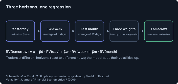
RV is realized volatility for the day. Despite its simplicity and without true long memory, simulations show that the model reproduces long memory, fat tails and self-similarity, and the empirical results show “remarkably good forecasting performance”.1 That makes it a standard benchmark in volatility forecasting.
What did the original data show?
For S&P 500 futures from January 1990 to July 2007 (4,344 daily observations), the estimated weights were 0.372 on yesterday, 0.343 on the weekly average and 0.224 on the monthly average, all highly significant. For USD/CHF the weights were 0.352, 0.323, 0.235; for Treasury-bond futures 0.039, 0.412 and 0.361, where the daily term was not significant.1 Out of sample, with the model re-estimated every day on a moving window of 1,000 observations, HAR beat the short-memory AR(1) and AR(3) at one-day, one-week and two-week horizons and performed about as well as a true long-memory ARFIMA model with far fewer parameters.1
How does it do on Bitcoin?
We measured daily realized volatility as the square root of the sum of squared hourly log returns within a UTC day, on Binance USD-M BTCUSDT from October 2020 to October 2026: 2,191 complete days, with a mean daily value of 2.6%. Then we forecast each next day with a 500-day rolling window, giving 1,669 out-of-sample forecasts, and compared three forecasts:2
| Forecast of next-day volatility | RMSE (percentage points) | MAE | R² of Mincer–Zarnowitz regression |
|---|---|---|---|
| Yesterday’s value | 1.31 | 0.96 | 0.246 |
| Mean of the last 22 days | 1.24 | 0.86 | 0.124 |
| HAR (three horizons) | 1.13 | 0.82 | 0.258 |
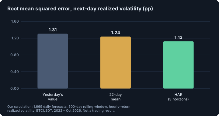
HAR cut the root-mean-squared error by 14% relative to yesterday’s value and by 9% relative to the monthly mean.2 The R² gain over yesterday’s value is small, since yesterday’s value already carries most of the signal, while the monthly mean has the lowest R²; HAR combines their strengths. Full-sample weights for Bitcoin were 0.306 on yesterday, 0.269 on the weekly and 0.294 on the monthly average, with a small intercept (0.34 percentage points).2
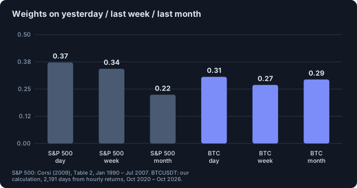
Compared with the S&P 500, Bitcoin puts a larger share on the long window and a smaller one on yesterday. The reading is that Bitcoin volatility has a longer memory in our data: a turbulent month stays relevant. That fits the slow decay of the autocorrelation of absolute returns on the same contract (0.16 after one day, 0.05 after twenty), described in Bitcoin’s fat tails and volatility clustering.
How could you use a volatility forecast?
- Stop distance. Express the stop in units of forecast daily volatility rather than a fixed number: if the forecast is 3% and the price is 80,000, one forecast “day” is about 2,400. The point is consistency across calm and turbulent periods; the paper does not test stops, and neither do we.
- Position size. Dividing a fixed risk amount by the stop distance automatically shrinks size when volatility is forecast to be high; see Kelly criterion and position size.
- Context. A higher forecast also means wider fills and more slippage when you need to exit.
What are the limits?
- The test measures volatility forecasts, not profits. We did not trade anything.
- Realized volatility from hourly returns is coarser than the tick-based measure Corsi used (his estimator uses 10-tick returns and a two-scale correction).1
- Seven years of one asset; weights change over time, which is why we re-estimated on a rolling window.
- Large jumps (the March 2020 crash is outside our sample, which starts in October 2020) are inherently hard to forecast; a regression on past volatility cannot see them coming.
This is educational material, not investment advice.
Related. Bitcoin’s fat tails and volatility clustering, Kelly criterion and position size.
Footnotes
-
Fulvio Corsi, “A Simple Approximate Long-Memory Model of Realized Volatility”, Journal of Financial Econometrics 7(2), 174–196 (2009); full text read: abstract, section 2 (model), section 3 (data, Table 2 weights, Table 5 out-of-sample forecasts). Data: USD/CHF December 1989 – December 2003; S&P 500 futures January 1990 – July 2007 (4,344 observations); T-bond futures January 1990 – October 2003. ↩ ↩2 ↩3 ↩4 ↩5 ↩6
-
Our calculation: Binance USD-M BTCUSDT hourly candles, 7 October 2020 to October 2026; daily realized volatility = √(sum of 24 squared hourly log returns) for days with all 24 hours (2,191 days); HAR regression of next-day value on daily value, 5-day mean and 22-day mean, re-estimated each day on the previous 500 observations; out-of-sample forecasts 1,669 (from about March 2022); error measures against the realized next-day value; R² from a Mincer–Zarnowitz regression of actual on forecast. Not a trading result. ↩ ↩2 ↩3 ↩4
Frequently asked questions
What is the HAR model of volatility?
HAR-RV is a simple regression: tomorrow’s realized volatility is explained by yesterday’s daily realized volatility, the average of the last 5 days and the average of the last 22 days. The three terms stand for traders with daily, weekly and monthly horizons.
How do you forecast Bitcoin volatility?
One practical way is to compute daily realized volatility as the square root of the sum of squared hourly returns, and regress the next day on the daily, 5-day and 22-day averages. In our test this gave a lower error than yesterday’s value or the monthly mean.
Is a volatility forecast the same as a price forecast?
No. The model predicts how large tomorrow’s move is likely to be, not whether it is up or down. Direction stays close to unpredictable.
How should I use a volatility forecast for stop-losses?
It can set a distance in units of expected daily movement instead of a fixed number, so stops are wider in turbulent periods and tighter in calm ones. Whether that improves results must be tested separately; the model alone does not show it.
Sources
- A Simple Approximate Long-Memory Model of Realized Volatility. Fulvio Corsi, Journal of Financial Econometrics 7(2), 174–196 (2009); full text read, 2009
This article is research, not investment advice. Results on history do not guarantee future results.