
- Short answer: in 58 liquid futures over 1965–2009 the sign of the past 12-month return predicted the sign of the next month’s return in every instrument, and a diversified rule-based portfolio had an annual Sharpe ratio above 1, with no trading costs deducted. That is the strongest published evidence for trend following, and it has limits.
- The rule is mechanical: go long if the past 12-month excess return is positive, short if negative, with each position sized to a constant volatility (40% a year per instrument in the paper).
- The effect lasted about a year and then partly reversed. The strategy earned most in extreme markets, and lost sharply when a crisis ended and trends reversed (March to May 2009).
- Later work argues much of the diversified portfolio’s alpha comes from volatility scaling, not momentum. And the study covers traditional futures, not crypto: treat it as a hypothesis for crypto, not a result.
Short answer. The most cited academic case for trend following is a 2012 paper by Tobias Moskowitz, Yao Hua Ooi and Lasse Heje Pedersen. Across 58 liquid futures, a security’s own past 12-month return predicted its next-month return, and a simple diversified portfolio built on that rule earned an annual Sharpe ratio above 1. It is real evidence. It is also evidence about commodities, currencies, equity indexes and bonds, without trading costs deducted, with the portfolio measured on 1985–2009 returns, and not about crypto.
What exactly did the study find?
The authors call the pattern “time series momentum” and describe it as “remarkably consistent across very different asset classes and markets”.1 The data are futures prices for 24 commodities, 12 currency pairs, nine developed equity indexes and 13 government bond futures, January 1965 to December 2009. The central results:
- The past 12-month excess return of each instrument was a positive predictor of its future return, and 12-month time series momentum profits were positive for every one of the 58 contracts.
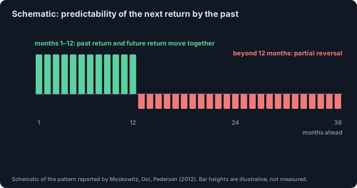
- Persistence lasted about a year and then partially reversed over longer horizons.
- A diversified portfolio of the strategies delivered, in the authors’ words, “substantial abnormal returns with little exposure to standard asset pricing factors”: an annual Sharpe ratio greater than one, roughly 2.5 times that of the equity market portfolio.1
How is the rule built?
The strategy is deliberately simple, which is why it is easy to check:
- For each instrument, look at the excess return over the past 12 months.
- If it is positive, go long for the next month; if negative, go short.
- Size the position inversely to the instrument’s recent volatility, so each position targets the same risk. The paper uses 40% annualized volatility per instrument.1
A numeric illustration (ours): if one future’s volatility is 20% a year, the 40% target means a position of 2× its capital; at 80% volatility the position is 0.5×. A calm market is levered up and a wild one is shrunk, so a single volatile instrument cannot dominate the portfolio.
When does trend following lose?
The paper is explicit about the weak spot. The portfolio did best in extreme markets, with large payoffs in both big rallies and big declines (the authors compare it to an option straddle on the market). But:
The ending of a crisis constitutes a sharp trend reversal that generates losses on a trend following strategy
Moskowitz, Ooi, Pedersen, “Time series momentum”, Journal of Financial Economics (2012)
They note large profits in the fourth quarter of 2008 and sharp losses in March, April and May of 2009, when the crisis ended.1 Trend following is a bet that today’s direction continues; it pays for that bet in choppy markets and at turning points. This is the same trade-off we describe in why backtests mislead: a smooth historical curve hides the periods where the rule is out of step with the market.
Who is on the other side?
Using weekly CFTC positioning data, the authors find speculators tend to be positioned with the trend and hedgers against it, and conclude that speculators profit from time series momentum at the expense of hedgers.1 On theory, they are cautious: the pattern fits sentiment stories of initial under-reaction and delayed over-reaction, but they also say they “cannot rule out the existence of a rational theory”. They also find it hard to fit existing behavioral models, for example because time series momentum is more strongly correlated across asset classes than the assets themselves.
What did later work challenge?
Kim, Tse and Wald re-examined the result and argued that the big alpha of the diversified portfolio is driven largely by volatility scaling, a risk-parity-style weighting, rather than by momentum itself: without volatility scaling, time series momentum and buy-and-hold had similar cumulative returns and alphas that were not significantly different.2 You do not need to take a side to draw the practical lesson. How you size positions is part of the strategy, and the headline Sharpe ratio belongs to the rule and the sizing together.
What does it mean for a crypto trader?
- Not tested here. None of the 58 instruments is a cryptocurrency, and the sample ends in 2009. For crypto, see the separate evidence on momentum and attention in our summary of Liu and Tsyvinski.
- Numbers are before costs. The instrument-level Sharpe ratios in the paper are labelled gross, and we found no deduction of trading costs in its headline results; futures trading costs, funding in perpetual contracts and slippage (what is slippage) come off the top.
- Prove it on your own sample. A 12-month rule has few independent signals per year: judging it needs the sample-size arithmetic in how many trades prove a strategy works, and a record of how many variants you tried.
- Plan for the drawdown. The rule is expected to lose at reversals. Decide your maximum tolerable loss in advance; the risk simulator shows what a run of losses does to an account.
This is educational material, not investment advice.
Footnotes
-
Moskowitz, T. J., Ooi, Y. H., Pedersen, L. H., “Time series momentum”, Journal of Financial Economics 104(2), 2012, pp. 228–250 (full text read). Data and results: sections 1–3 (58 instruments; January 1965 to December 2009; positive 12-month profits for every contract; persistence for about a year with partial reversal), section 4 (portfolio alpha, sample January 1985 to December 2009; Sharpe above one, about 2.5 times the equity market; extreme-market “smile”; losses at the end of the 2008–09 crisis), section 6 (speculators and hedgers). Position size 40%/σ and the gross Sharpe ratios of the instrument-level figure are from section 4 and Figure 2. ↩ ↩2 ↩3 ↩4 ↩5
-
Kim, A. Y., Tse, Y., Wald, J. K., “Time series momentum and volatility scaling”, Journal of Financial Markets 30, 2016, pp. 103–124. We relied on the published bibliographic record and a summary of its abstract; we did not read the full paper, and its specific figures are not quoted here. ↩
Frequently asked questions
What is time series momentum?
It is the tendency of an asset’s own past return to predict its future return. In the Moskowitz–Ooi–Pedersen study, the past 12-month excess return of each of 58 futures was a positive predictor of its return over the following month.
How does a time series momentum strategy work?
For each instrument and month, go long if the excess return over the past 12 months is positive and short if it is negative, scaling each position to a constant ex ante volatility so instruments are comparable.
How long does time series momentum last?
The study finds persistence for about 12 months that partially reverses over longer horizons, consistent with under-reaction followed by delayed over-reaction.
Does trend following work in crypto?
This study does not test it: its sample is commodity, currency, equity-index and government-bond futures from 1965 to 2009. Whether the pattern holds in crypto needs its own out-of-sample test, with costs.
Sources
- Time series momentum. Tobias J. Moskowitz, Yao Hua Ooi, Lasse Heje Pedersen. Journal of Financial Economics 104(2), 228–250, 2012, 2012
- Time series momentum and volatility scaling. Abby Y. Kim, Yiuman Tse, John K. Wald. Journal of Financial Markets 30, 103–124, 2016, 2016
This article is research, not investment advice. Results on history do not guarantee future results.